Figure 2.14a Figure 2.14b
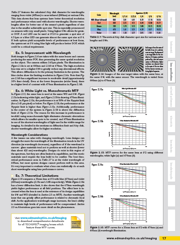
Each image is from the center of
the field of view of a multi element
star target. The elements of
a star target allow for the visualization
of changing resolution
produced by a lens and camera
system in all directions. Higher
resolutions are observed closer
to the center of the star where
the lines become narrower, producing
higher frequencies.
White Light Diffraction MTF
0 150
75
Spatial Frequency in Cycles per mm
Contrast (%)
100
90
80
70
60
50
40
30
20
10
0
470nm Illumination Diffraction MTF
75
0 150
Spatial Frequency in Cycles per mm
Contrast (%)
100
90
80
70
60
50
40
30
20
10
0
470nm Illumination Diffraction MTF
75
0 150
Spatial Frequency in cycles per mm
Contrast (%)
100
90
80
70
60
50
40
30
20
10
0
405nm Illumination Diffraction MTF
0 150
75
Spatial Frequency in Cycles per mm
Contrast (%)
100
90
80
70
60
50
40
30
20
10
0
www.edmundoptics.co.uk/imaging 17
introduction fundamentals lens specifications real world performance telecentricity lens mechanics lens selection guide
Table 2.7 features the calculated Airy disk diameter for wavelengths
ranging from violet (405nm) to near-infrared (880nm) at various f/#s.
This data shows that lens systems have better theoretical resolution
and performance when used with shorter wavelengths. Shorter wavelengths
allow for better use of the sensor’s pixels regardless of size
due to the smaller achievable spot size. This is especially pronounced
on sensors with very small pixels. Using higher f/#s allows for greater
DOF. A red LED can be used at f/2.8 to generate a spot size of
4.51μm or a blue LED can generate almost the same spot size at f/4.
If both options yield acceptable levels of performance at best focus,
the system set at f/4 using blue light will produce better DOF, which
could be a critical requirement.
uu Ex. 5: Improvement with Wavelength
Both images in Figure 2.14 are taken with the same lenses and camera
producing the same FOV, thus presenting the same spatial resolution
on the object. The camera utilizes 3.45μm pixels. The illumination in
Figure 2.14a is set at 660nm and 2.14b at 470nm. The high-resolution
lens was set to a higher f/# to greatly reduce any aberrational effects.
This allows diffraction to be the primary limitation in the system. The
blue circles show the limiting resolution in Figure 2.14a. Note that Figure
2.14b has a significant increase in resolvable detail (approximately
50% finer detail). Even at the lower frequencies (wider lines), there
is a higher level of contrast with 470nm illumination in Figure 2.14b.
uu Ex. 6: White Light vs. Monochromatic MTF
In Figure 2.15, the same lens is used at the same WD and f/#. Figure
2.15a is showing white light, and Figure 2.15b is showing 470nm illumination.
In Figure 2.15a, the performance is at 50% of the Nyquist limit
(for a 3.45 μm pixel) or below. For Figure 2.15b, the performance at the
Nyquist limit is higher than Figure 2.15a. Additionally, performance
in the center of the system in Figure 2.15b is above the diffraction
limit of Figure 2.15a. The reason for this increase in performance is
twofold: using monochromatic light eliminates chromatic aberrations
which allows for smaller spots to be created, and 470nm illumination
is one of the shortest wavelengths of light used in the visible range for
imaging. As detailed in the sections on diffraction limit and Airy disk,
shorter wavelengths allow for higher resolution.
Wavelength Considerations
A few issues can arise with changing wavelength. Lens designs can
struggle the more the wavelength of the illumination trends in the UV
direction (as wavelength decreases), regardless of if the waveband is
narrow: glass materials tend not to perform as well at shorter (lower
than about 425 nm) wavelengths. Designs do exist in this region of
the spectrum, but they are often limited in capabilities, and the exotic
materials used require the lens build to be costlier. The best theoretical
performance seen in Table 2.7 is at the violet wavelength of
405nm, but most system designs cannot perform well in this area.
It’s very important to evaluate what a lens can realistically do at such
short wavelengths using lens performance curves.
uu Ex. 7: Theoretical Limitations
Figure 2.16 compares a 35mm lens at f/2 with blue (470nm) and violet
(405nm) wavelengths (2.16a and 2.16b respectively). While Figure 2.16a
has a lower diffraction limit, it also shows that the 470nm wavelength
yields higher performance at all field positions. The effect here is increased
when the lens is used at the extremes of its design capabilities
for f/# and WD (detailed in Section 2.5 on MTF). Another wavelength
issue that can greatly affect performance is related to chromatic focal
shift. As the application’s wavelength range increases, the lens’s ability
to maintain high levels of performance will be compromised. Section
3.5 on Aberrations goes into more detail on the phenomenon.
Visit www.edmundoptics.co.uk/imaging
to download comprehensive datasheets
for all TECHSPEC® imaging lenses which
feature these MTF curves.
Color Wavelength
(nm)
Aperture (f/#)
f/1.4 f/2.8 f/4 f/8 f/16
NIR (Near-Infrared) 880 3.01 6.01 8.59 17.18 34.36
Red 660 2.25 4.51 6.44 12.88 25.77
Green 520 1.78 3.55 5.08 10.15 20.30
Blue 470 1.61 3.21 4.59 9.17 18.35
Violet 405 1.38 2.77 3.95 7.91 15.81
Table 2.7: Theoretical Airy disk diameter spot size for various wavelengths
and f/#s.
Figure 2.14: Images of the star target taken with the same lens, at
the same f/#, with the same sensor. The wavelength is varied from
660nm (a) to 470nm (b).
Figure 2.15a
Figure 2.15b
Figure 2.15: MTF curves for the same lens at f/2 using different
wavelengths; white light (a) and 470nm (b).
Figure 2.16a
Figure 2.16b
Figure 2.16: MTF curves for a 35mm lens at f/2 with 470nm (a) and
405nm (b) wavelength illumination.
/imaging
/imaging