illumination cameras microscopy / objectives filters / accessories liquid lens / specialty telecentric fixed focal length resource guide
Figure 3.17a
DOF: 20 lp/mm, f/2.8, 200mm Focus
100
90
80
70
60
50
40
30
20
10
0
0.00 200.0 400.0
Working Distance Shift (mm)
TS 5.50mm
TS 4.00mm
TS 0.00mm
DOF: 20 lp/mm, f/4.0, 200mm Focus
100
90
80
70
60
50
40
30
20
10
0
0.00 200.0 400.0
Working Distance Shift (mm)
Contrast (%)
Contrast (%)
TS 5.50mm
TS 4.00mm
TS 0.00mm
Figure 3.17b
24 +44(0) 1904 788600 | Edmund Optics® targets Figure 3.18a
DOF: 20 lp/mm, f/2.8, 200mm Focus
100
90
80
70
60
50
40
30
20
10
0
0.00 200.0 400.0
Working Distance Shift (mm)
TS 5.50mm
TS 4.00mm
TS 0.00mm
DOF: 20 lp/mm, f/2.8, 500mm Focus
100
90
80
70
60
50
40
30
20
10
0
0.00 500.0 1000.0
Working Distance Shift (mm)
Contrast (%)
Contrast (%)
TS 5.50mm
TS 4.00mm
TS 0.00mm
Figure 3.18b
How f/# Affects DOF
Changing the f/# of a lens changes DOF, shown in Figure 3.19. For
each configuration shown in Figure 3.19 there are two bundles of rays.
The bundle represented by dotted black lines shows how well the
lens is focused. As an object moves away from the best focus position
(where the dotted lines cross), object details move into a wider area
of the cone. The wider the spread of the cone, the more the image
blurs into the surroundings. The f/# of the lens controls how quickly
the cone expands and how much information or detail is blurred together
at a given distance. Figure 3.19a shows a lens with a shallow
DOF, where Figure 3.19b shows a lens with a large DOF.
Maximum Blur Allowable
Maximum Blur Allowable
Best Focus To Obtain Desired Resolution
Best Focus To Obtain Desired Resolution
Figure 3.19a
Figure 3.19b
The red cone in Figure 3.19 is an angular representation of the system
resolution. Where the lines of the red cone and dotted black cone
intersect defines the total range of the DOF. The lower the f/#, the
faster the black dotted lines expand, and the lower the DOF.
As details get smaller (represented by a smaller red cone), the bundles
in Figure 3.19a and 3.19b move closer together. Eventually, increasing
the f/# too much causes smaller details to blur due to reaching the
lens diffraction limit, since the limiting resolution of the lens is inversely
proportional to f/#. This limitation means that while increasing
the f/# will always increase the DOF, the minimum resolvable
feature size (even at best focus) increases. For more information on
the diffraction limit and its relationship to f/#, see Section 2.4. Using
short wavelengths helps to salvage some of this resolution. Learn
more about how wavelength affects system performance in Section
Section 3.4: Depth of Field and
Depth of Focus
Due to similarity in name and nature, depth of field (DOF) and
depth of focus are commonly confused concepts. To simplify the
definitions, DOF concerns the image quality of a stationary lens as
an object is repositioned, whereas depth of focus concerns a stationary
object and a sensor’s ability to maintain focus for different
sensor positions, including tilt.
Depth of Field
The DOF of a lens is its ability to maintain a desired amount of image
quality (spatial frequency at a specified contrast), without refocusing,
if the object position is moved closer and farther from the plane of
best focus. DOF also applies to objects with complex geometries or
features of different height. As an object is placed closer to or farther
than the set focus distance of a lens, the object blurs and both
resolution and contrast suffer. As such, DOF only makes sense if it is
defined with an associated resolution and contrast. Several targets
can be used to directly measure and benchmark an imaging system’s
DOF; these targets are detailed in Section 12.
Resolution and DOF
“Does this lens have good DOF?” It is difficult to quantify without
specifying an object detail size or image space frequency. The smaller
the detail, the higher the spatial frequency needed, and the smaller
the DOF the lens can produce. A DOF curve can be used to see how
a lens performs over a given depth at a specific detail’s size. These
graphs not only consider theoretical limitations associated with the
f/# setting, but also the aberrational effects of the lens design.
In Figure 3.17, contrast values (y-axis) are seen over a WD range (x-axis)
at a fixed frequency of 20lp/mm (image detail). Note the difference
in DOF between Figure 3.17a, which is set at f/2.8, and Figure 3.17b,
which is set at f/4. Also note that there is more usable DOF beyond
the best focus than between the best focus and the lens, due to magnification
decreasing. The graphs themselves contain different colored
lines denoting different sensor positions. These types of asymmetric
DOF curves are common in fixed focal length lenses.
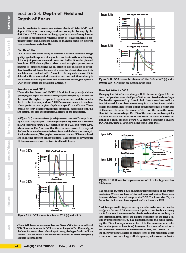
Figure 3.18 features the same lens as Figure 3.17a but at a different
WD. Note an increase in DOF occurs at longer WDs. Eventually, as
the lens focuses at objects infinitely far away, the hyperfocal condition
occurs. This condition is reached at the distance in which everything
appears in equal focus.
DOF
DOF
Low f/# (Large Aperture)
Lens Mount
Flange Distance
Image / Sensor
ω
ω
DOF
DOF
Low f/# (Large Aperture)
High f/# (Small Aperture)
Image / Sensor Image / Sensor
ω
ω
Figure 3.19: Geometric representation of DOF for high and low
f/# lenses.
Figure 3.17: DOF curves for a lens at f/2.8 (a) and f/4 (b).
Figure 3.18: DOF curves for a lens at f/2.8 at 200mm WD (a) and at
500mm WD (b). Note (b) has a much larger scale.