1
ξ 6.8 Cutoff = λ × (f/#)
227lp/mm 12.4m feature size
Group 5, Element 3
145lp/mm
67lp/mm
Spatial Frequency in Cycles per mm
TS 0.00mm
Diff. Limit
www.edmundoptics.co.uk/imaging 41
resource guide telecentric liquid lens/specialty objectives cameras illumination targets
fixed focal length filters/accessories microscopy /
The example on the previous page also assumes that the exact camera/
sensor has not yet been chosen, therefore making the optics the
limiting component in the imaging system. If a camera sensor had been
chosen prior to the lens, the lens would need to be able to resolve the
pixel size of the sensor in use.
Continuing from the example on the previous page, if a camera had
been chosen with the Sony IMX250 sensor with 3.45μm pixels, using
Equation 6.6 the image space resolution can be found as 144.9lp/mm.
Section 6.4: Sensors and Lenses
Looking at the MTF curve, the lens achieves >40% contrast, which is
more than enough for most applications. However, using the same calculation
as in Equation 6.7 to scale into object space, 3.45μm pixels only
corresponds to a 45μm object, meaning the sensor would be the limiting
component in the system, as the lens is capable of 26μm object space
resolution.
All of these considerations must be made when determining the
proper lens for a given application in order to fi nd the optimal solution
to a machine vision problem.
Imaging at the Nyquist Frequency
It can be tempting to image at what is called the Nyquist frequency,
which is defi ned in Equation 6.5, from Section 6.3. However, this is generally
not a good idea, as it implies that the feature that is being observed
falls on exactly one pixel. Were the imaging system to shift by a half a
pixel, the object of interest would fall between two pixels, and would
blur out completely. For this reason, imaging at the Nyquist frequency is
not recommended. Assuming no sub-pixel interpolation is being used,
imaging at half of the Nyquist frequency is generally recommended, as
this will allow the feature of interest to always take up at least two pixels.
Another assumption that is often improperly made is that a lens is
not appropriate for use with a particular camera unless it has substantial
(>20%) contrast at the Nyquist frequency of the sensor that it is being
used with. This is not the case. As previously mentioned, imaging at the
Nyquist limit is ill-advised, and can create several problems. The entire
system needs to be looked at to determine whether a lens is appropriate
for a given camera sensor or not, and this is often dependent on the application.
The following section describes what happens in an imaging
system when they are used at or near the Nyquist frequency, and the
consequences on overall system resolution.
Understanding the interplay between camera sensors and imaging
lenses is a vital part of designing and implementing a machine vision
system. The optimization of this relationship is often overlooked, and
the impact that it can have on the overall resolution of the system is
large. An improperly paired camera/lens combination could lead to
wasted money on the imaging system. Unfortunately, determining
which lens and camera to use in any application is not always an easy
task: more camera sensors (and as a direct result, more lenses) continue
to be designed and manufactured to take advantage of new manufacturing
capabilities and drive performance up. These new sensors present
a number of challenges for lenses to overcome and make the correct
camera to lens pairing less obvious.
The fi rst challenge is that pixels continue to get smaller. While
smaller pixels typically mean higher system-level resolution, this
is not always the case once the optics used are taken into account.
In a perfect world, with no diff raction or optical errors in a system,
resolution would be based simply upon the size of a pixel and the size
of the object that is being viewed (see Section 2.2: Resolution). To briefl y
summarize, as pixel size decreases, the resolution increases. This increase
occurs as smaller objects can be fi t onto smaller pixels and still
be able to resolve the spacing between the objects, even as that spacing
decreases. This is an oversimplifi ed model of how a camera sensor detects
objects, not taking noise or other parameters into account.
Lenses also have resolution specifi cations, but the basics are not quite
as easy to understand as sensors since there is nothing quite as concrete
as a pixel. However, there are two factors that ultimately determine
the contrast reproduction (modulation transfer function, or MTF) of a
particular object feature onto a pixel when imaged through a lens: diffraction
and aberrational content. Diff raction will occur any time light
passes through an aperture, causing contrast reduction (more details in
Section 2.4: The Airy Disk and Diff raction Limit). Aberrations are errors
that occur in every imaging lens that either blur or misplace image information
depending on the type of aberration, as described in Section
3: Real World Performance on pages 20-28. With a fast lens (≤f/4), optical
aberrations are most often the cause for a system departing from “perfect”
as would be dictated by the diff raction limit; in most cases, lenses
simply do not function at their theoretical cutoff frequency (ξCutoff ), as
dictated by Equation 6.8.
To relate this equation back to a camera sensor, as the frequency of
pixels increases (pixel size goes down), contrast goes down - every lens
will always follow this trend. However, this does not account for the real
world hardware performance of a lens. How tightly a lens is toleranced
and manufactured will also have an impact on the aberrational content
of a lens and the real-world performance will diff er from the nominal,
as-designed performance. It can be diffi cult to approximate how a realworld
lens will perform based on nominal data, but tests in a lab can
help determine if a particular lens and camera sensor are compatible.
One way to understand how a lens will perform with a certain sensor
is to test its resolution with a USAF 1951 bar target. Bar targets
are better for determining lens/sensor compatibility than star targets,
as their features line up better with square (and rectangular) pixels.
113lp/mm, 24.8m feature size
Group 4, Element 3
Contrast 24.8%
Contrast 8.8%
33lp/mm
Contrast 55.3%
Contrast: 33.6%
72lp/mm
Contrast 48%
Contrast: 24.6%
Sensor
a) ON Semiconductor
MT9P031
2.2μm
/ Nyquist Nyquist
Modulus of the OTF
1.0
0.9
0.8
0.7
0.6
0.5
0.4
0.3
0.2
0.1
0.0
0 22.7 45.4 68.1 90.8 113.5 136.2 158.9 181.6 204.3 227
b) Sony
ICX655
3.45μm
c) ON Semiconductor
KAI-4021
7.4μm
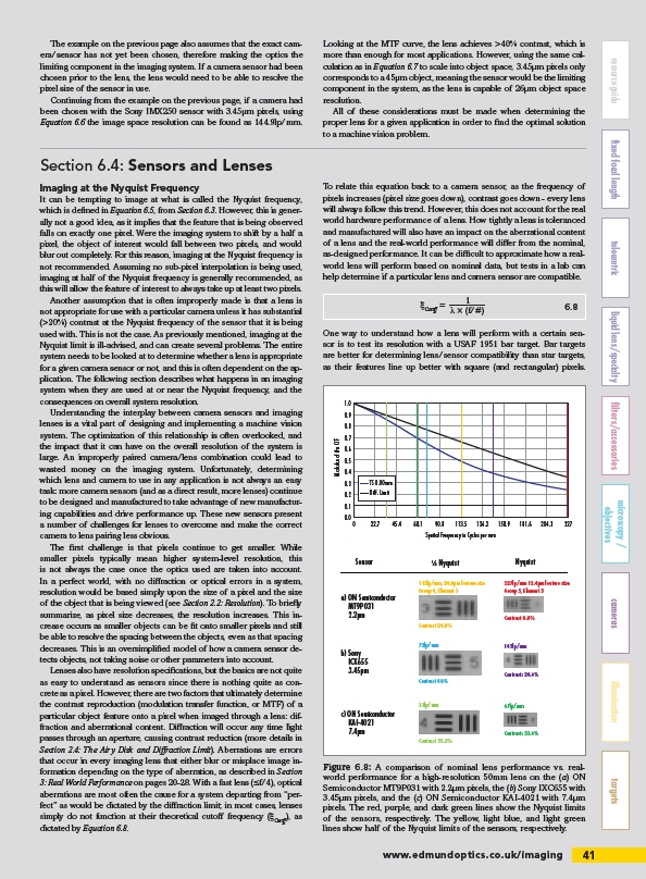
Figure 6.8: A comparison of nominal lens performance vs. realworld
performance for a high-resolution 50mm lens on the (a) ON
Semiconductor MT9P031 with 2.2μm pixels, the (b) Sony IXC655 with
3.45μm pixels, and the (c) ON Semiconductor KAI-4021 with 7.4μm
pixels. The red, purple, and dark green lines show the Nyquist limits
of the sensors, respectively. The yellow, light blue, and light green
lines show half of the Nyquist limits of the sensors, respectively.
/imaging