Section 2.6: MTF Curves and Lens Performance
MTF: f/2.8, 150mm WD, 12mm FL
100
90
80
70
60
50
40
30
20
10
0
0.0 75.0
10μm 5μm
Spatial Frequency in Cycles per mm
Pixel Size:
Contrast (%)
150.0
MTF: f/2.8, 150mm WD, 12mm FL
100
90
80
70
60
50
40
30
20
10
0
0.0 75.0
10μm 5μm
Spatial Frequency in Cycles per mm
Pixel Size:
Contrast (%)
150.0
MTF: f/2.8, 150mm WD, 12mm FL
100
90
80
70
60
50
40
30
20
10
0
0.0 75.0
10μm 5μm
Spatial Frequency in Cycles per mm
Pixel Size:
Contrast (%)
150.0
MTF: f/2.8, 200mm WD, 16mm FL
100
90
80
70
60
50
40
30
20
10
0
0.0 75.0
10μm 5μm
Spatial Frequency in Cycles per mm
Pixel Size:
Contrast (%)
150.0
www.edmundoptics.co.uk/imaging 15
introduction fundamentals lens specifications real world performance telecentricity lens mechanics lens selection guide
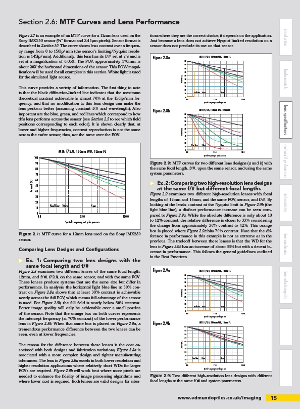
Figure 2.7 is an example of an MTF curve for a 12mm lens used on the
Sony IMX250 sensor (2/3” format and 3.45μm pixels). Sensor format is
described in Section 10. The curve shows lens contrast over a frequency
range from 0 to 150lp/mm (the sensor’s limiting/Nyquist resolution
is 145lp/mm). Additionally, this lens has its f/# set at 2.8 and is
set at a magnification of 0.05X. The FOV, approximately 170mm, is
about 20X the horizontal dimensions of the sensor. This FOV/magnification
will be used for all examples in this section. White light is used
for the simulated light source.
This curve provides a variety of information. The first thing to note
is that the black diffraction-limited line indicates that the maximum
theoretical contrast achievable is almost 70% at the 150lp/mm frequency,
and that no modification to this lens design can make the
lens perform better (assuming constant f/# and wavelength). Also
important are the blue, green, and red lines which correspond to how
this lens performs across the sensor (see Section 2.5 to see which field
positions corresponding to each color). It is shown clearly that, at
lower and higher frequencies, contrast reproduction is not the same
across the entire sensor, thus, not the same over the FOV.
MTF: f/2.8, 150mm WD, 12mm FL
100
90
80
70
60
50
40
30
20
10
0
0.0 75.0
10μm 5μm
Spatial Frequency in Cycles per mm
Pixel Size:
Contrast (%)
150.0
Comparing Lens Designs and Configurations
uu Ex. 1: Comparing two lens designs with the
same focal length and f/#
Figure 2.8 examines two different lenses of the same focal length,
12mm, and f/#, f/2.8, on the same sensor, and with the same FOV.
These lenses produce systems that are the same size but differ in
performance. In analysis, the horizontal light blue line at 30% contrast
on Figure 2.8a shows that at least 30% contrast is achievable
nearly across the full FOV, which means full advantage of the sensor
is used. For Figure 2.8b, the full field is nearly below 30% contrast.
Better image quality will only be achievable over a small portion
of the sensor. Note that the orange box on both curves represents
the intercept frequency (at 70% contrast) of the lower performance
lens in Figure 2.8b. When that same box is placed on Figure 2.8a, a
tremendous performance difference between the two lenses can be
seen, even at lower frequencies.
The reason for the difference between these lenses is the cost associated
with both designs and fabrication variations; Figure 2.8a is
associated with a more complex design and tighter manufacturing
tolerances. The lens in Figure 2.8a excels in both lower resolution and
higher resolution applications where relatively short WDs for larger
FOVs are required. Figure 2.8b will work best where more pixels are
needed to enhance the fidelity of image processing algorithms and
where lower cost is required. Both lenses are valid designs for situations
where they are the correct choice; it depends on the application.
Just because a lens does not achieve Nyquist limited resolution on a
sensor does not preclude its use on that sensor.
Figure 2.8a
Figure 2.8b
uu Ex. 2: Comparing two high-resolution lens designs
at the same f/# but different focal lengths
Figure 2.9 examines two different high-resolution lenses with focal
lengths of 12mm and 16mm, and the same FOV, sensor, and f/#. By
looking at the lens’s contrast at the Nyquist limit in Figure 2.9b (the
light blue line), a distinct performance increase can be seen compared
to Figure 2.9a. While the absolute difference is only about 10
to 12% contrast, the relative difference is closer to 33% considering
the change from approximately 30% contrast to 42%. This orange
box is placed where Figure 2.9a hits 70% contrast. Note that the difference
in performance in this example is not as extreme as in the
previous. The tradeoff between these lenses is that the WD for the
lens in Figure 2.9b has an increase of about 33% but with a decent increase
in performance. This follows the general guidelines outlined
in the Best Practices.
Figure 2.7: MTF curve for a 12mm lens used on the Sony IMX250
sensor.
Figure 2.8: MTF curves for two different lens designs (a and b) with
the same focal length, f/#, upon the same sensor, and using the same
system parameters.
Figure 2.9a
Figure 2.9b
Figure 2.9: Two different high-resolution lens designs with different
focal lengths at the same f/# and system parameters.
/imaging