Minimum Wavefront
Radius of Curvature Planar Wavefront
z =
z
z = zR
w(z) = 2w0
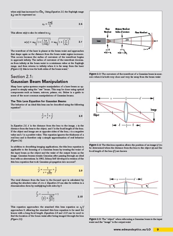
Figure 2.3: The curvature of the wavefront of a Gaussian beam is nearzero
when it is both very close and very far away from the beam waist
s’
www.edmundoptics.eu/LO 9
when w(z) has increased to √2w0. Using Equation 2.5, the Rayleigh range
(zR) can be expressed as:
This allows w(z) to also be related to zR:
The wavefront of the laser is planar at the beam waist and approaches
that shape again as the distance from the beam waist region increases.
This occurs because the radius of curvature of the wavefront begins
to approach infi nity. The radius of curvature of the wavefront decreases
from infi nity at the beam waist to a minimum value at the Rayleigh
range, and then returns to infi nity when it is far away from the laser
(Figure 2.3); this is true for both sides of the beam waist,3
Section 2.1:
Gaussian Beam Manipulation
Many laser optics systems require manipulation of a laser beam as opposed
to simply using the “raw” beam. This may be done using optical
components such as lenses, mirrors, prisms, etc. Below is a guide to
some of the most common manipulations of Gaussian beams.
The Thin Lens Equation for Gaussian Beams
The behavior of an ideal thin lens can be described using the following
equation2:
In Equation 2.8, s’ is the distance from the lens to the image, s is the
distance from the lens to the object, and f is the focal length of the lens.
If the object and image are at opposite sides of the lens, s is a negative
value and s’ is a positive value. This equation ignores the thickness of a
real lens and is therefore only a simple approximation of real behavior
(Figure 2.4).
In addition to describing imaging applications, the thin lens equation is
applicable to the focusing of a Gaussian beam by treating the waist of
the input beam as the object and the waist of the output beam as the
image. Gaussian beams remain Gaussian after passing through an ideal
lens with no aberrations. In 1983, Sidney Self developed a version of the
thin lens equation that took Gaussian propagation into account2:
The total distance from the laser to the focused spot is calculated by
adding the absolute value of s to s’. Equation 2.9 can also be written in a
dimensionless form by multiplying both sides by f:
This equation approaches the standard thin lens equation as zR/f
approaches 0, allowing the standard thin lens equation to be used for
lenses with a long focal length. Equations 2.9 and 2.10 can be used to
fi nd the location of the beam waist after being imaged through the lens
(Figure 2.5).
Planar
Wavefront
z = 0
w(z) = w0
s
-f f
s’
Laser
Object
Image
Figure 2.4: The thin lens equation allows the position of an image (s’) to
be determined when the distance from the lens to the object (s) and the
focal length of the lens (f ) are known
2.6
2.7
2.8
2.9
2.10
s
wo wo’
Figure 2.5: The ”object” when refocusing a Gaussian beam is the input
waist and the “image” is the output waist
/LO