Instrument
Table 16.2: Reasonable spatial frequency ranges of a white light interferometer
with interchangeable objectives and an atomic force microscope5
Distorted Wavefront
www.edmundoptics.eu/LO 55
a reference optic in the other (Figure 16.7). The length of the reference
arm is varied by translating the reference optic through some range.
WLI and AFM have overlapping spatial frequency ranges and can both
be utilized for measuring sub-angstrom surface roughness of superpolished
surfaces (Table 16.2), which instrument is better is dependent on
the spatial frequency range being measured,5 It is widely accepted that
optics intended to be used in the visible spectra do not need to be measured
beyond ~2000 cycles/mm, which is ideal for WLI. However, for
optics intended to be used in the UV spectra the higher spatial frequency
range of the AFM may be required. The AFM can also measure lower
spatial frequencies (as seen in Table 16.2), but other factors make AFM
less production friendly. Due to longer measurement times, AFM has an
extreme sensitivity to temperature fl uctuations and external vibrations.
Therefore, AFM is better suited for the controlled environment of a test
lab while WLI is better suited for a factory setting.
Section 16.5:
Shack-Hartmann Wavefront Sensors
A Shack-Hartmann wavefront sensor (SHWFS) measures the transmitted
and refl ected wavefront error of an optical component or system
with high dynamic range and accuracy. The SHWFS has become very
popular due to its ease of use, fast response, relatively low cost, and ability
to work with incoherent light sources.
The wavefront of an optical wave is a surface over which the wave has a
constant phase. Wavefronts are perpendicular to the direction of propagation,
therefore collimated light has a planar wavefront and converging
or diverging light has a curved wavefront (Figure 16.8). Aberrations in optical
components lead to wavefront errors, or distortions in transmitted
or refl ected wavefronts. By analyzing transmitted and refl ected wavefront
error, the aberrations and performance of an optical component
can be determined.
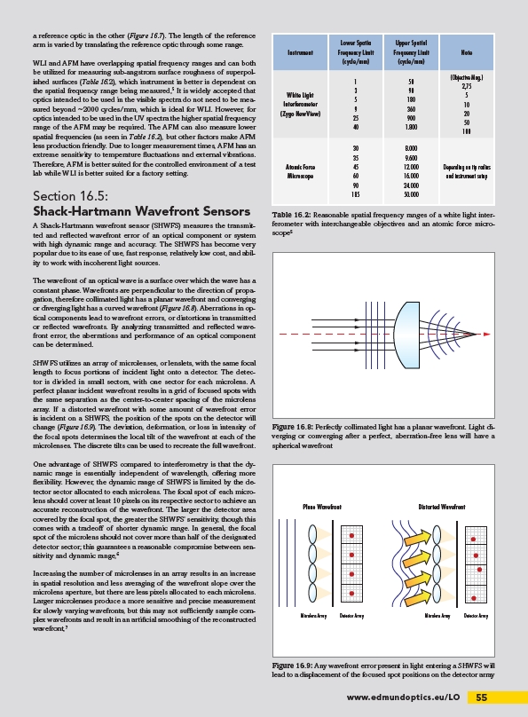
SHWFS utilizes an array of microlenses, or lenslets, with the same focal
length to focus portions of incident light onto a detector. The detector
is divided in small sectors, with one sector for each microlens. A
perfect planar incident wavefront results in a grid of focused spots with
the same separation as the center-to-center spacing of the microlens
array. If a distorted wavefront with some amount of wavefront error
is incident on a SHWFS, the position of the spots on the detector will
change (Figure 16.9). The deviation, deformation, or loss in intensity of
the focal spots determines the local tilt of the wavefront at each of the
microlenses. The discrete tilts can be used to recreate the full wavefront.
One advantage of SHWFS compared to interferometry is that the dynamic
range is essentially independent of wavelength, off ering more
fl exibility. However, the dynamic range of SHWFS is limited by the detector
sector allocated to each microlens. The focal spot of each microlens
should cover at least 10 pixels on its respective sector to achieve an
accurate reconstruction of the wavefront. The larger the detector area
covered by the focal spot, the greater the SHWFS’ sensitivity, though this
comes with a tradeoff of shorter dynamic range. In general, the focal
spot of the microlens should not cover more than half of the designated
detector sector; this guarantees a reasonable compromise between sensitivity
and dynamic range,6
Increasing the number of microlenses in an array results in an increase
in spatial resolution and less averaging of the wavefront slope over the
microlens aperture, but there are less pixels allocated to each microlens.
Larger microlenses produce a more sensitive and precise measurement
for slowly varying wavefronts, but this may not suffi ciently sample complex
wavefronts and result in an artifi cial smoothing of the reconstructed
wavefront,7
Figure 16.8: Perfectly collimated light has a planar wavefront. Light diverging
or converging after a perfect, aberration-free lens will have a
spherical wavefront
Lower Spatia
Frequency Limit
(cycle/mm)
Upper Spatial
Frequency Limit
(cycle/mm)
Note
White Light
Interferometer
(Zygo NewView)
1
3
5
9
25
40
50
90
180
360
900
1.800
(Objective Mag.)
2,75
5
10
20
50
100
Atomic Force
Microscope
30
35
45
60
90
185
8.000
9.600
12.000
16.000
24.000
50.000
Depending on tip radius
and instrument setup
Plane Wavefront
Microlens Array Detector Array
Microlens Array Detector Array
Figure 16.9: Any wavefront error present in light entering a SHWFS will
lead to a displacement of the focused spot positions on the detector array
/LO