illumination cameras microscopy / objectives filters / accessories liquid lens / specialty telecentric fixed focal length resource guide
At this point different cameras must be evaluated to achieve this
performance. To keep costs minimal, it is important to start with as
small a resolution as possible. In today’s machine vision world, this
is often 0,3 MP, or VGA resolution. The aspect ratio of the sensor is
4:3. However, the FOV that is needed is 1:1; this means that the small
dimension of the sensor (480 pixels) will need to correspond to the
35mm FOV, and the larger dimension will float. There will likely be
some wasted pixels.
Because 480 pixels are going to be divided among 35 mm of space,
each pixel corresponds to 73 μm in object space. This camera is certainly
insufficient for this application, and it is required to have a resolution
about 3X better. Running through the math again with a 1600 × 1200
sensor with 4,5 μm pixels, each pixel now takes up 29 μm, which is sufficient.
But how does this correspond to image space with a camera and
lens? At this point, the system needs to be linked to the magnification.
Since this 1600 × 1200 sensor has pixels that correspond to
4,5 μm in size, the dimensions are 7,2 mm × 5,4 mm. Using Equation
6.4, the magnification required is 0,15X. It is now possible to use this
magnification to not only determine which lens is needed, but to also
determine the resolution needed for the imaging system to properly
reproduce the image of the barcode.
Since a sensor has been chosen, Equation 6.3 from Section 6.2 can
now be used to determine the focal length of the lens. Using Equation
6.3, the focal length required based on the 200 mm WD is 30 mm.
However, the magnification required (0,15X) can be achieved with
a 25 mm lens from 230 mm away; in this example this is sufficient.
Now a preliminary lens has been chosen, but can it work based on the
resolution required?
The resolution required in object space is 5 lp/mm. Converting this
into image space by dividing by the magnification, 33 lp/mm is required
to view the object properly. This number needs to be checked
against the Nyquist frequency of the sensor and the modulation
transfer function (MTF) of the lens that is being used. See Section 2.2:
Resolution for more information on the Nyquist frequency. Equation 6.5
describes the Nyquist frequency of a sensor as:
where s is the pixel size. Using Equation 6.5, a sensor with 4,5 μm pixels
has a Nyquist frequency of 111l p/mm. Because this is larger than
the required 33 lp/mm, this camera is a good choice. Note that this is
because there are three pixels covering our feature so the resolution is
unsurprisingly at about 3X less than the Nyquist frequency. This math
was included for completeness.
Figure 6.6 shows the MTF curve for the 25 mm C Series Fixed Focal
Length Lens used at a WD of 166 mm (for more information on how to
read an MTF curve, see Section 2.5: Modulation Transfer Function). The
curve shows that the 25 mm lens achieves 83% contrast at 33 lp/mm,
which is more than sufficient.
0
0 15.0 30.0 45.0 60.0 75.0 90.0 105.0 120.0 135.0 150.0
Spatial Frequency in Cycles per mm
Contrast
1.0
0.5
Generally, 20% is the minimum contrast value required for an imaging
lens to resolve an object; this lens has more than enough contrast at
targets this resolution.
40 +44 (0) 1904 788600 | Edmund Optics® 1
Nyquist Frequency = 2 × s 6.5
Figure 6.6: MTF curve of a 25 mm C Series Fixed Focal Length Lens
that achieves a more than sufficient resolution for this example.
This is just the tip of the iceberg when selecting a lens for a given
application. MTF is affected by several factors (explained in detail in
Section 2.6: MTF Curves and Lens Performance), and oftentimes is not
straightforward. The following section goes into detail on looking specifically
at a lens and how well it matches to a camera.
The Changing Performance of a Lens
Lens suppliers are able to provide bespoke MTF curves based on how
the lens is used. In the barcode example above, the MTF of the 25 mm
lens was referenced to determine if it had sufficient contrast reproduction
for the barcode that it was imaging. Now, we will expand on this
using a different example, but with the same lens, to show how things
do not always work out as intended.
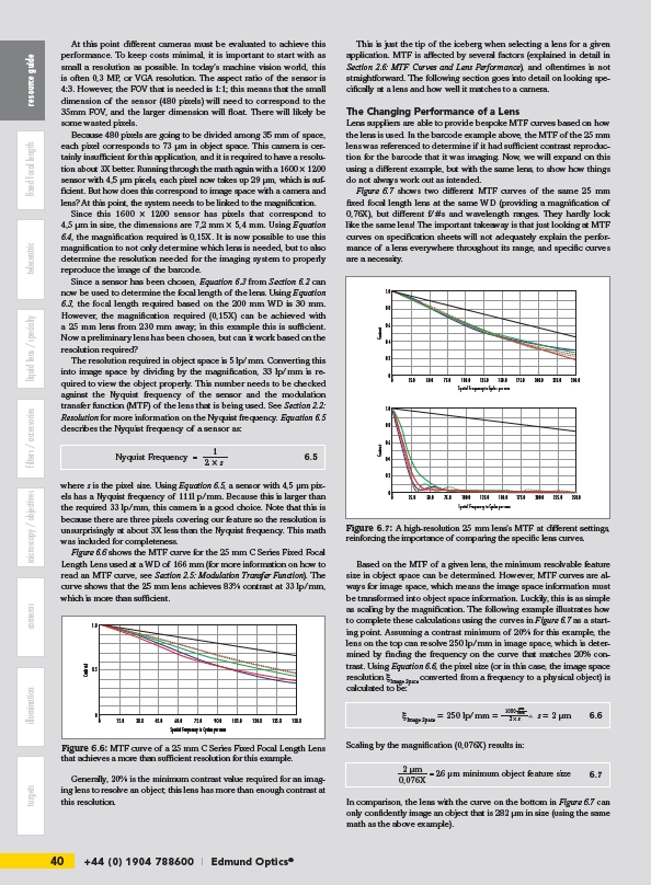
Figure 6.7 shows two different MTF curves of the same 25 mm
fixed focal length lens at the same WD (providing a magnification of
0,76X), but different f/#s and wavelength ranges. They hardly look
like the same lens! The important takeaway is that just looking at MTF
curves on specification sheets will not adequately explain the performance
of a lens everywhere throughout its range, and specific curves
are a necessity.
Contrast Spatial Frequency in Cycles per mm
0
0 25.0 50.0 75.0 100.0 125.0 150.0 175.0 200.0 225.0 250.0
Spatial Frequency in Cycles per mm
1.0
0.8
0.6
0.4
0.2
1.0
0.8
0.6
0.4
0.2
0
0 25.0 50.0 75.0 100.0 125.0 150.0 175.0 200.0 225.0 250.0
Contrast
Figure 6.7: A high-resolution 25 mm lens’s MTF at different settings,
reinforcing the importance of comparing the specific lens curves.
Based on the MTF of a given lens, the minimum resolvable feature
size in object space can be determined. However, MTF curves are always
for image space, which means the image space information must
be transformed into object space information. Luckily, this is as simple
as scaling by the magnification. The following example illustrates how
to complete these calculations using the curves in Figure 6.7 as a starting
point. Assuming a contrast minimum of 20% for this example, the
lens on the top can resolve 250 lp/mm in image space, which is determined
by finding the frequency on the curve that matches 20% contrast.
Using Equation 6.6, the pixel size (or in this case, the image space
resolution ξImage Space converted from a frequency to a physical object) is
calculated to be:
μm
mm s = 2 μm
ξ Space = 250 lp/mm = 1000
6.6 Image 2 × s
Scaling by the magnification (0,076X) results in:
= 26 μm minimum object feature size 6.7
2 μm
0,076X
In comparison, the lens with the curve on the bottom in Figure 6.7 can
only confidently image an object that is 282 μm in size (using the same
math as the above example).