illumination cameras microscopy / objectives filters / accessories liquid lens / specialty telecentric fixed focal length resource guide
Figure 3.24a Figure 3.24b
f/2.8 f/5.6
Pixel
Center of Image
2 Adjacent Pixels
Corner of Image
12.5m Tilt
25m Tilt
Pixel
Center of Image
12.5m Tilt
25m Tilt
2 Adjacent Pixels
Corner of Image
Figure 3.25a
f/2.8
Corner
Center
Diff. Limit
Best Focus on axis.
0.32 deg image tilt for 25m center-to-corner shift
0 150
75
Spatial Frequency in Cycles per mm
Contrast (%)
100
90
80
70
60
50
40
30
20
10
0
Figure 3.25b
Contrast (%)
100
90
80
70
60
50
40
30
20
10
0
f/5.6
Corner
Center
Diff. Limit
Best Focus on axis.
0. 32 deg image tilt for 25m center-to-corner shift
26 +44 (0) 1904 788600 | Edmund Optics® targets Section 3.5: Aberrations
Optical aberrations are performance deviations from a perfect, mathematical
model. It is important to note that they are not caused by
any manufacturing fl aws - physical, optical, nor mechanical. Rather,
they are inherent in lens design and are due to diff raction, refraction,
and the wave nature of light. As such, there is no “perfect” lens. Effects
from various aberrations in a lens design are ultimately seen in
performance and aff ect MTF, spot size, telecentricity, DOF, and others.
Aberration theory is an abstract and complex subject. However,
understanding how aberrations aff ect performance is important for
success with an application.
Common Aberration Types
While aberration theory is a vast subject, basic knowledge of a few
fundamental concepts can ease understanding: spherical aberration,
astigmatic aberrations, fi eld curvature, and chromatic aberration.
Spherical Aberration
Spherical aberration refers to rays focusing at diff erent distances
depending on where they interact with the lens and is a function of
aperture size. To describe spherical aberration, the incident angle of
light must be known. This angle occurs where light rays strike the
curved surface of a lens and is the angle between the ray and the
surface. The steeper the incident angle, the more the light will be refracted
(Figure 3.26). Figure 3.26 shows that as the parallel rays in object
space collide with the lens, the incident angle increases the farther
up they hit on the lens’s surface. Image quality from lenses with
large apertures (small f/#s) are more likely to suff er from spherical
aberration, because of this larger angle of incidence. Lenses that
suff er from spherical aberration can be improved by increasing the
f/# by closing the iris, but there is a limit to how much this improves
image quality. Closing the iris too much causes diff raction to limit
performance sooner (see diff raction limit in Section 2.4). Optical designs
that include high-index glass or additional elements are used
to correct spherical aberration in a fast (small f/#) lens; these designs
reduce the amount of refraction at each surface and, with it,
the amount of spherical aberration. However, this increases the size,
weight, and cost of the lens assembly.
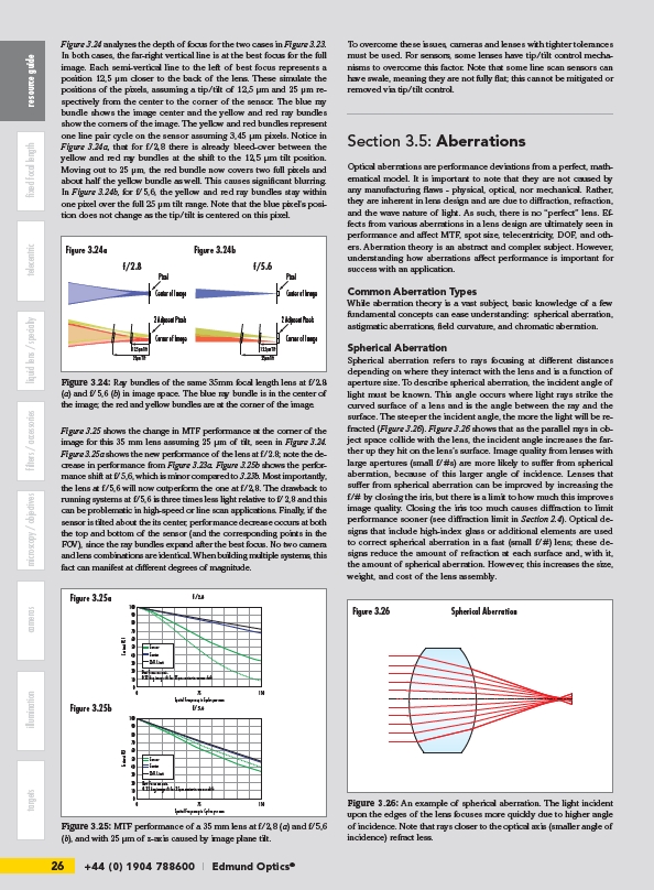
Figure 3.24 analyzes the depth of focus for the two cases in Figure 3.23.
In both cases, the far-right vertical line is at the best focus for the full
image. Each semi-vertical line to the left of best focus represents a
position 12,5 μm closer to the back of the lens. These simulate the
positions of the pixels, assuming a tip/tilt of 12,5 μm and 25 μm respectively
from the center to the corner of the sensor. The blue ray
bundle shows the image center and the yellow and red ray bundles
show the corners of the image. The yellow and red bundles represent
one line pair cycle on the sensor assuming 3,45 μm pixels. Notice in
Figure 3.24a, that for f/2,8 there is already bleed-over between the
yellow and red ray bundles at the shift to the 12,5 μm tilt position.
Moving out to 25 μm, the red bundle now covers two full pixels and
about half the yellow bundle as well. This causes signifi cant blurring.
In Figure 3.24b, for f/5,6, the yellow and red ray bundles stay within
one pixel over the full 25 μm tilt range. Note that the blue pixel’s position
does not change as the tip/tilt is centered on this pixel.
Figure 3.25 shows the change in MTF performance at the corner of the
image for this 35 mm lens assuming 25 μm of tilt, seen in Figure 3.24.
Figure 3.25a shows the new performance of the lens at f/2.8; note the decrease
in performance from Figure 3.23a. Figure 3.25b shows the performance
shift at f/5,6, which is minor compared to 3.23b. Most importantly,
the lens at f/5,6 will now outperform the one at f/2,8. The drawback to
running systems at f/5,6 is three times less light relative to f/2,8 and this
can be problematic in high-speed or line scan applications. Finally, if the
sensor is tilted about the its center, performance decrease occurs at both
the top and bottom of the sensor (and the corresponding points in the
FOV), since the ray bundles expand after the best focus. No two camera
and lens combinations are identical. When building multiple systems, this
fact can manifest at diff erent degrees of magnitude.
To overcome these issues, cameras and lenses with tighter tolerances
must be used. For sensors, some lenses have tip/tilt control mechanisms
to overcome this factor. Note that some line scan sensors can
have swale, meaning they are not fully fl at; this cannot be mitigated or
removed via tip/tilt control.
Figure 3.26 Spherical Aberration
Figure 3.26: An example of spherical aberration. The light incident
upon the edges of the lens focuses more quickly due to higher angle
of incidence. Note that rays closer to the optical axis (smaller angle of
incidence) refract less.
Figure 3.24: Ray bundles of the same 35mm focal length lens at f/2.8
(a) and f/5,6 (b) in image space. The blue ray bundle is in the center of
the image; the red and yellow bundles are at the corner of the image.
75
0 150
Spatial Frequency in Cycles per mm
Figure 3.25: MTF performance of a 35 mm lens at f/2,8 (a) and f/5,6
(b), and with 25 μm of z-axis caused by image plane tilt.