illumination cameras microscopy / objectives filters / accessories liquid lens / specialty telecentric fixed focal length resource guide
uu Ex. 3: Comparing different f/#s of the same
35 mm lens design
Figure 2.10 features the MTF for a 35 mm lens design using white
light at f/4 (a) and f/2 (b). The yellow line on both graphs shows the
diffraction-limited contrast at the Nyquist limit for Figure 2.10a while
the blue line denotes the lowest actual performance at the Nyquist
limit of the same lens at f/4 in Figure 2.10a. While the theoretical limit
of Figure 2.10b is far higher, the performance is much lower. This example
shows that higher f/#s can reduce aberrational effects, greatly
increasing lens performance, even if the theoretical performance
limit is greatly reduced. The primary tradeoff of stopping down the
lens (increasing the f/#), besides resolution, is less light throughput.
uu Ex. 4: The Effect of Changing Working Distance
on MTF
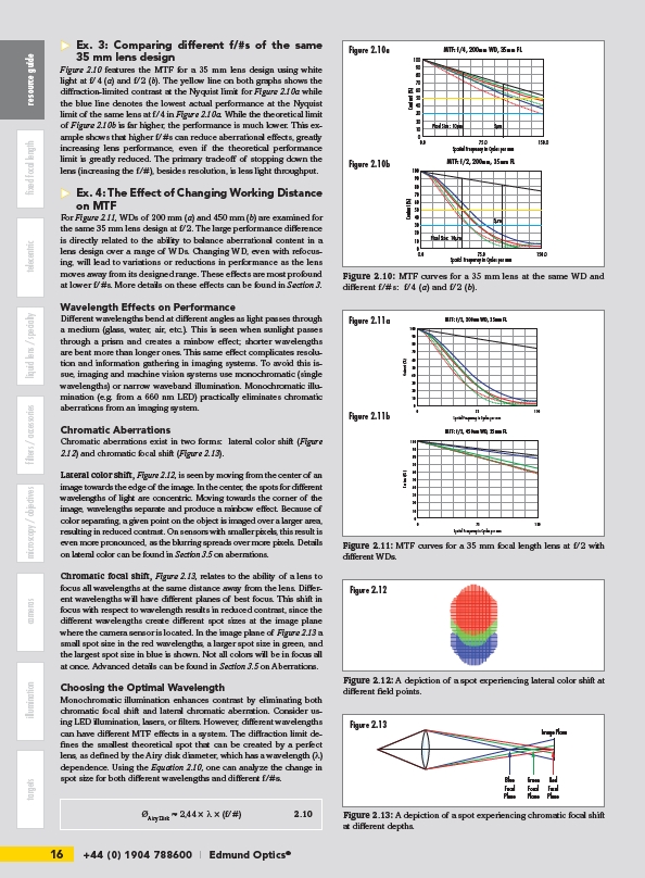
For Figure 2.11, WDs of 200 mm (a) and 450 mm (b) are examined for
the same 35 mm lens design at f/2. The large performance difference
is directly related to the ability to balance aberrational content in a
lens design over a range of WDs. Changing WD, even with refocusing,
will lead to variations or reductions in performance as the lens
moves away from its designed range. These effects are most profound
at lower f/#s. More details on these effects can be found in Section 3.
Wavelength Effects on Performance
Different wavelengths bend at different angles as light passes through
a medium (glass, water, air, etc.). This is seen when sunlight passes
through a prism and creates a rainbow effect; shorter wavelengths
are bent more than longer ones. This same effect complicates resolution
and information gathering in imaging systems. To avoid this issue,
imaging and machine vision systems use monochromatic (single
wavelengths) or narrow waveband illumination. Monochromatic illumination
(e.g. from a 660 nm LED) practically eliminates chromatic
aberrations from an imaging system.
Chromatic Aberrations
Chromatic aberrations exist in two forms: lateral color shift (Figure
2.12) and chromatic focal shift (Figure 2.13).
Lateral color shift, Figure 2.12, is seen by moving from the center of an
image towards the edge of the image. In the center, the spots for different
wavelengths of light are concentric. Moving towards the corner of the
image, wavelengths separate and produce a rainbow effect. Because of
color separating, a given point on the object is imaged over a larger area,
resulting in reduced contrast. On sensors with smaller pixels, this result is
even more pronounced, as the blurring spreads over more pixels. Details
on lateral color can be found in Section 3.5 on aberrations.
Chromatic focal shift, Figure 2.13, relates to the ability of a lens to
focus all wavelengths at the same distance away from the lens. Different
wavelengths will have different planes of best focus. This shift in
focus with respect to wavelength results in reduced contrast, since the
different wavelengths create different spot sizes at the image plane
where the camera sensor is located. In the image plane of Figure 2.13 a
small spot size in the red wavelengths, a larger spot size in green, and
the largest spot size in blue is shown. Not all colors will be in focus all
at once. Advanced details can be found in Section 3.5 on Aberrations.
Choosing the Optimal Wavelength
Monochromatic illumination enhances contrast by eliminating both
chromatic focal shift and lateral chromatic aberration. Consider using
LED illumination, lasers, or filters. However, different wavelengths
can have different MTF effects in a system. The diffraction limit defines
the smallest theoretical spot that can be created by a perfect
lens, as defined by the Airy disk diameter, which has a wavelength (λ)
dependence. Using the Equation 2.10, one can analyze the change in
spot size for both different wavelengths and different f/#s.
16 +44 (0) 1904 788600 | Edmund Optics® targets MTF: f/4, 200mm WD, 35mm FL
100
90
80
70
60
50
40
30
20
10
0
Pixel Size: 10μm 5μm
0.0 75.0 150.0
Spatial Frequency in Cycles per mm
Contrast (%)
MTF: f/2, 200mm, 35mm FL
100
90
80
70
60
50
40
30
20
10
0
Pixel Size: 10μm
5μm
0.0 75.0 150.0
Spatial Frequency in Cycles per mm
Contrast (%)
Figure 2.10a
Figure 2.10b
Figure 2.10: MTF curves for a 35 mm lens at the same WD and
different f/#s: f/4 (a) and f/2 (b).
MTF: f/2, 200nm WD, 35mm FL
0 75
Spatial Frequency in Cycles per mm
Contrast (%)
100
90
80
70
60
50
40
30
20
10
0
150
MTF: f/2, 450nm WD, 35mm FL
0 75 150
Spatial Frequency in Cycles per mm
Contrast (%)
100
90
80
70
60
50
40
30
20
10
0
Figure 2.11a
Figure 2.11b
Figure 2.11: MTF curves for a 35 mm focal length lens at f/2 with
different WDs.
Figure 2.12
Figure 2.12: A depiction of a spot experiencing lateral color shift at
different field points.
Image Plane
Blue
Focal
Plane
Green
Focal
Plane
Red
Focal
Plane
Figure 2.13
Figure 2.13: A depiction of a spot experiencing chromatic focal shift
at different depths.
ØAiry Disk ≈ 2,44 × λ × (f/#) 2.10